Being Made Whole in Bankruptcy

In our discussions in our Managing Corporate Turnarounds class during our financial restructuring session, I got to thinking about what it would take to be made whole in a bankruptcy scenario. While the hard math will tell you that it is impossible in the short term (EV = 80, Net Debt = 100), I began to think back to the PIK and using a high yield to restore value in the future. So my question became this: If I hold the debt of an insolvent company, what can I negotiate to help me restore value? The most obvious solution is to renegotiate the terms of my debt which will probably result in me taking a haircut (discount) on the principal or face value of my debt. However, we’ve acknowledged that in scenarios where people become riskier, obviously the company’s related securities should bear a higher return. So my question then evolved to: If I have to take a discount of X percent, what additional spread Y would I have to earn in order to be made whole in N years. It turns out:

FV x (1 + kd) ^ N = FV x (1 – X) x (1 + kd + Y) ^ N

However, this assumes that you can break even with (or more accurately, catch up to) where your security would have been if the company had not defaulted to begin with. After playing with these numbers, however, it was quite clear that even with a small discount (say 20% discount), the spread Y had to be astronomically (unreasonably) higher in order to have any chance of being made whole relative to the standard debt, so I thought it would be unrealistic not to include a factor which accounts for the value lost:

FV x (1 + kd) ^ N = FV x (1 – X) x (1 + kd + Y) ^ N + Value Lost

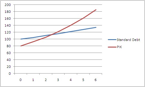
In trying to understand what these numbers mean, I looked at Value Lost / FV as a proxy for the default rate of this type of security in distress which is obviously closely tied to the actual economic circumstances of the company. In the graph, it is reflected by the distance between the Standard Debt curve and the PIK (Realistic) curve.

Also, Y can probably be determined by looking at the spread between similar bonds with different credit ratings (dropping from BBB to C for instance).

X is reflective of the economic scenario (so if EV was 80 and Net Debt was 100, X would be 20%). It is also reflective of the negotiations, as well as considering a discount in order to liquidate the current assets of the company.

Another problem is also that once a company switches from PIK to cash sweep, its risk profile drops and it stops earning high yields, dropping the return on capital and therefore making it impossible to “catch up”. Also, a bank which was happy to finance your debt will not be interested in converting neither into a mezzanine structure better suited for hedge funds nor into equity.

This model is similar to the VC model of predicting the failure rate using the discount rate except in reverse. It is also similar to the interest rate parity (IRP) model and boot strapping by using compounding to determine where you would have / should have been otherwise as a benchmark for where you are going.

I guess the real lesson is that bankruptcy is really expensive and that being made whole in this scenario is difficult, regardless of the financial engineering and patience, although these two factors can be used to ease the pain.

Managing Corporate Turnarounds - Part II

Wednesday

Often when things go wrong, people are inclined to fire the management. However, in the real world, things are hardly ever that simple. Firing management, like anything in turnarounds, is decided on whether or not this action will speed up or slow down the turnaround. Besides packages given to executives on exit, there is also a great deal of institutional knowledge that they take with them. There is a counter balance to understanding the value they bring through their experience versus the inertia they create against the changes required. This is particularly true in SMEs as well as family owned enterprises where the institutional knowledge is often not formalized (pricing mechanics, customer relationships etc.)

Also, with the separation of the chairman and CEO roles, it is possible that a power divide coupled with an inappropriate strategy may have smart people being told to chase bad strategies. One remedy which is often used is an immunity period: the idea that employees in a turnaround situation have a window of opportunity to identify any potential problems. This allows an honest analysis of problems without reprimand and realigns expectations (Are we going to make the numbers? Are our margins as good as we expect? Are we doing things right? Are we doing the right things?) Because a new team is put into place to fix previously created problems, it is not appropriate to assign current problems to new management. However, eventually, whether or not these issues were created by you initially you will inevitably begin to wear them if you don’t fix them soon enough or don’t manage expectations of the company and all stakeholders.

Thursday

Like in any business strategy, there are two major things to keep in mind in a restructuring: operations and financing. For operations, it is necessary to check if the overall business strategy works (are people buying your product and do you have a viable business) and if you are able to profitably deliver (are our margins good or are we chasing low quality customers). Also from a financing perspective, it is important to understand the liquidity constraints of the enterprise. For example, what is an appropriate financing structure to keep the company alive while providing adequate and appropriate protection and returns to current and new capital providers?

One such useful tool is the paid-in-kind (PIK) security. It is a type of mezzanine high yield debt that doesn’t pay a coupon. Typically, these types of securities return 14 to 17%. They return higher than senior debt because they are subordinated but they don’t require cash payments which allow the company to maintain its liquidity for short period of time when it’s heavily cash strapped. However, what usually happens is this is coupled with a cash sweep. To use a structure like this in this circumstance is tantamount to saying: “We understand you are strapped for cash now, so you don’t have to pay us immediately, but we want an appropriate return for taking this risk that’s more similar to equity if things recover. However, we still want to be paid sooner rather than later and when you have any excess cash, you will give us everything you have and we’ll consider you less risky and ratchet down your interest rate to reflect the change in risk.”

Managing Corporate Turnarounds

This week, I’m taking a block week course (one week intensive following the 10 week standard course period) at LBS: Managing Corporate Turnarounds. So far this course has actually been really interesting, with us looking at business cases for salvaging distressed companies and learning about the mechanics and considerations of struggling businesses.

Unlike my undergraduate strategy course, which I nicknamed “doom and gloom” because the distressed companies in our cases never seemed to recover, this course talks about different cases that were successfully turned around using a variety of different techniques to improve operational efficiencies and use financial tools like LBOs to capture the upside.

We’ve also had great guest speakers come talk about their specific experiences and their perspective on different aspects of turning companies around (shedding assets for cash, improving operations, recovering debt, how to identify target companies etc.) One of our requirements in class is to summarize some key learnings from the class, and in a similar fashion to the Latin America study tour which had a similar component, I plan on using this blog to jot a few notes for me to recall later as I compile my thoughts:

Monday

In turning a company around, it is important to understand where control lies. Since equity is flirting with bankruptcy, it may lose control to the debt holders. Some debt investors may be holding “grenades”, the intent to liquidate their holdings ASAP when a trigger event happens (broken covenants, default etc), and may not be interested in salvaging the company, even if there is potential to recover equity value because they just want to unwind their positions.

Companies need to have good strategies when it comes to M&A, otherwise they can fall victim of a vicious cycle: accretive acquisitions increase EPS (albeit in an inorganic manner) and can give false impressions of growth, which could potentially boost the P/E multiple. A higher P/E multiple gives the company expensive equity which it can use as a better transaction currency for buying other companies (low P/E) and still be accretive. This is a vicious cycle if the M&A is not well integrated with substantial delivery of synergies and/or overpays for targets. This typically occurs in new industries where there are a limited number of potential buyers (targets with low P/Es as there is no other mechanism for exit) and the industry is consolidating into larger players (large strategic buyers displace financial buyers niche shopping).

Another version of the problem above is when companies which are asset-light use M&A as a backdoor for raising leverage. Services companies cannot raise leverage in a traditional manner because they have neither hard assets nor collateral to borrow against, so they can acquire companies which have higher leverage ratios to boost their own ratios. Also, this type of reckless acquisition can divert focus from the core business. In turning around companies which have fallen along this path, one of the immediate remedies is to spin off non-core assets for cash.

Tuesday

When you are on the buyside for any company (not just distressed companies for turnaround), it is important to have multiple targets in the pipe, not just for the more obvious negotiation leverage points, but to prevent yourself from getting too much deal heat over one deal and to avoid negotiating against yourself and your emotions.

Negotiating a transaction involves much more than a “price”. There are terms of payment, the structure of the compensation, workouts, milestones, terms and conditions. A price which is seemingly too high can be restructured to be paid out overtime so that the undiscounted amount remains the same, but the risk and cash outflows can be spread over a longer period with the appropriate covenants and milestones.

FEI Competition

Apparently, our final round presentation for the Financial Executives International Case Competition is now available online. Unfortunately, I can't embed it into the blog, but I can include the link below:

http://www.feicanada.org/cfo-tv.php?vid=22&page=2

Enjoy!

Bridge to Value

One graph I've seen which I thought was clever was a breakdown of change in EV. This brings together many other details I've learned about M&A, LBO's and transactions in general.

Previously, I mentioned a framework for PE deal success, but it is easy to cut into more detail if necessary and really define and put a mathematical value to "synergies".

For example: After a transaction, we've increased sales by 21%. How does that affect EV? Well on one hand, you've immediately realized a 21% increase in revenue. After you account for associated costs with that increase in revenue (ie. You've sold more widgets, but it still costs you money to make those widgets), what do your future growth prospects look like as a result of this new growth (ie. Should you trade at a higher multiple? Have you gone from "boring" to "exciting"? Or is it just general market conditions?)

Previously, you had:

Market Cap = $100
Shares outstanding = 100
Price per share = $1

Debt = $100 (@ 5%)
Excess Cash = 0

EV = $200

Revenue - $100
COGS - $40
GPM = $60

Op Ex - $20
EBITDA = $40

DA - $10
EBIT = $30

Interest = $5

Tax = 40%

NOPAT = $18
NI = $15

Therefore:

EPS = 15 cents

P/E = ($1/$0.15) = 6.67x

EV/EBITDA = ($200/$40) = 5.00x

Let's tell a story: The 21% increase comes from opening a new line of products. You are selling 10% more products by introducing a new product line and this new product line actually increases your revenue per unit (across the board) by 10% (110% x 110% = 121%). All margins are the same.

What should we do? Bring everything down to the EBITDA level:

Now:
Revenue - $121
COGS - $44 (10% more products at same costs)

GPM = $77

Op Ex - $22

EBITDA = $55

DA - $10
EBIT = $47

Interest = $5

Tax = 40%

NOPAT = $28.20
NI = $25.20

EPS = 25.20c

(Magic happens - Which we will explain shortly)

New Price per share = $1.80

Market Cap = $1.80 x 100 shares = $180
Debt = $100
EV = $280

P/E = ($1.80) / ($0.2520) = 7.14x
EV/EBITDA = ($280 / $55) = 5.09x

Analysis:
So a lot is going on. The price of the equity and the enterprise has changed, but how can we do a cross section such that we know exactly where all the value is being driven from?

How much of this value is because of leverage (hint, we didn't change amount of leverage)?
How much of this value is simply because we are operationally better?
How much of this value is because we have a "brighter future" (better growth prospects)?

Step 1: Value from leverage arbitrage:
No change = 0

Step 2: Value from "synergies":
Total EBITDA level changes: $40 to $55 or $15
At a multiple of 5.00x (previous multiple), value increased is $75

Step 3: Value from "Brighter future"
Brighter future (higher multiple) due to either market conditions or expected future growth:
$55 at 5.00x versus at 5.09x = $55 x (5.09 - 5.00x) = $5

Total value created: $75 + $5 = $80 (note total increase in value of EV / Market Cap)

Next step, look closer at Step 2:
Change of $40 to $55 is created by:
$21 in Revenue (Price +10%, Volume +10%)
$4 in COGS (Volume + 10%)
$2 in Opex (Volume +10%)

For a $21 increase in revenue, keeping margins constant we would have expected an increase of:
$8.4 in COGS (40% of revenue) and $4.2 in Opex (20% of revenue). COGS is lower by $4.4 and Opex is lower by $2.2 versus what is expected.

Note we mentioned we can sell products for 10% more across the board.
This created value for existing product base (at EBITDA level) of
$110 - $40 - $20 or $50 versus $40 creating $10 of additional EBITDA level value (makes sense, increase topline growth by 10% without changing expenses / sales volumes results in increase of EBITDA by 10% of revenue)

Also, selling an additional 10% at old price we would expect:
$10 (additional sales) - COGS ($4) - Opex ($2) or $4

But selling new products at new price: Gain $1 (similar to math shown above)

Total change in EBITDA: $10 + $4 + $1 = $15
At 5.00x
$55 or ($10 + $1) x 5.00x of EV is generated from selling at a higher price
$20 ($4 x 5.00x) of EV is generated from selling new products (higher volume)

Above is what the bridge would look like if a PE firm had 60% ownership and management had 40%.

Note, this framework is iterative and can be applied across multiple product lines to help do a break out and sum of the parts analysis for companies to see where value is hidden in undervalued divisions.

Also note that as an interesting aside, if you were actually to build out a proper DCF model of this (using some basic business assumptions holding margins constant etc.), your short term growth rate would have to be adjusted upwards in order to come to the same intrinsic valuation that would justify the higher multiple.

YCIF – London Chapter Inaugural Event

Yesterday, the Young Canadians in Finance organized their inaugural event in London at the Royal Automobile Club. The guest speaker was from the Canadian High Commission and spoke on the strong relationship between the UK and Canada and how Canada’s focus on increasing value added exports such as talent in the financial services sector was helping to improve Canada’s name abroad, especially in the light of our strength in the recent financial crisis.

The RAC was a beautiful club and it was nice to meet with fellow Canadians on this side of the pond. It was also surprising what a small world it is, as some of the people I had met had worked with some of my fellow Rotman students back on Bay Street at Canadian banks as recently as this summer.




My friend, Mathieu Bouthillier, has been a driving force for organizing YCIF’s presence in London, the first chapter outside of North America. He’s got a great line up of events including a series of guest speakers and social events which will be happening later this month and in March which I am looking forward to and will certainly attend.

It’s amazing some of the contacts you make and what you can learn just by having conversations with intelligent hardworking people with similar interests and it was a pleasure to be a yesterday’s event.

Islamic Finance – Executive 3 Day Program

Today, I presented remotely from London at the Islamic Finance Program, hosted at Rotman for the Executive Program in partnership with Bennett Jones. This was the final component of our Islamic Finance ICP. The team lead by Walid included myself, Arash, Shahzad, Khaled, Kashif and Noureen and we presented our materials to the executive program participants.

With the rise of Islamic finance, I’ve had some interesting conversations with people I’ve met while on exchange at LBS regarding Sharia compliant financial structures such as the various types of sukuks we’ve been analyzing.

Our spread analysis drove quite a bit of interest for people who were interested in what a Sharia compliant structure would yield and the market conditions for doing such an issuance. Even before our presentation, I had the opportunity to answer some basic questions regarding the pricing spread between Islamic instruments versus conventional.

ICP Islamic Finance - "Conventional" Analysis

This morning we had a working session for our ICP - Islamic Finance with some lawyers, a corporate banker and professors. The two teams presented their analysis of the conventional financing structure of the primary security instruments used to finnace our projects. Under this conventional analysis, we looked at the costs of capital and the associated terms related to these types of paper with the intent of understanding the requirements need to make them Sharia compliant.

We also had great explanation from a senior lawyer regarding the structuring and "asset-based" (versus "asset-backed") nature of nominating (rather than selling) assets under a Special Purpose Vehicle (SPV) in order to comply with the necessary requirements of Islamic finance. We had considered the capital gains implications of a sale leaseback transaction, as well as understood how an asset and capital intense infrastucture project would look similar under an adjusted EV to EBITDAR metric regardless of the off-balance sheet financing that may potentially be required.

We have a solid understanding of the work requirements due before our next meeting in early January (before I fly off for London). We also had an opportunity to fire questions back at the professionals in the room in terms to learn what were the appropriate resources for generating comparables for analysis and benchmarking of our theoretical capital structures based on similar Sharia compliant instruments and current market conditions.

Some of the best advice we got:

• Understand the difference between "asset backed" versus "asset based" and how that affects your ability to issue Sharia compliant instruments
• Be aware of tax implications of capital gains/losses in a sale leaseback transaction
• Like any financial security, understand the key characteristics of seniority and expected return for a sukuk issuance and understand market appetite for these structured products

DCF

With summer recruiting coming up for first years in the next few months and with many of our second year finance courses requiring us to do some form of valuation (Corp Fin, Financial Management, Mergers and Acquisitions, Business Analysis and Valuation etc.), I thought it might be useful to post an "academic" quality discounted cash flow model as a reference.

There are some basic comments in the cells which explain some of the assumptions.

Discounted Cash Flow Model

Discounted Cash Flow Guide

For a more advanced version of forecasting (including working capital schedule and depreciation schedule), check out my Chapters LBO model.

Multi-Factor Models – Applying the Lessons Learned from the Numbers

In Finance 1 last year, we were introduced to the idea of multi-factor models (MFM) originally explained by Fama and French as an alternative to the traditional Capital Asset Pricing Model (CAPM) for assessing systematic risk. Additional factors include small versus big (SML) and value versus growth (HML).

In our Business Analysis and Valuation class, we discussed a merger case in which a large company acquired a smaller company. We talked about what would be the best way to approximate beta. The method I used (which was the best method I could conceive, I’d be happy to hear criticism or suggestions otherwise) was to weight the betas by market cap and take an average.

However, there was some discussion about the fact that one entity was much smaller than the other. While we were having a conversation of what that would actually mean, I would suggest a mathematical method for expressing the quantitative effect of size, using FF’s MFM.

1. 1. Express both company’s re as a three factor MFM
   Re1 – RFR = beta1 (Rm – RFR) + betas1 (SMB) + betav1 (HML)
   Re2 – RFR = beta2 (Rm – RFR) + betas2 (SMB) + betav2 (HML)
2. Take the larger company’s size beta and apply it to the smaller entity
   betasnew = betas2
3. Recalculate re for both entities
   Re1new – RFR = beta1 (Rm – RFR) + betasnew (SMB) + betav1 (HML)
   Re2new – RFR = beta2 (Rm – RFR) + betasnew (SMB) + betav2 (HML)
4. Take a weighted average (by market cap) as the expected return of the combined entity

By taking the larger company’s size beta for both, what you are saying is that you expect the smaller company to have the size “characteristics” of the larger entity. I might even be more appropriate to add the size factors (Would that be appropriate? As the MFM is a linear regression, is it appropriate to add these factors?) and use that for new return on equity for each entity as it relates to the combined entity.

betasnew = betas1 + betas2

While there are some significant assumptions which are required for this to work, it is the best solution I can conjure based on information given. I would really appreciate any additional ideas for creating a more robust model.

Abnormal Earnings Method – Not Entirely Useless

When we were introduced to the Abnormal Earnings method in Business Analysis and Valuation, I was decomposing the math formula which constructs the value of the equity. As far as I was concerned, it didn’t really tell us anything we didn’t already know through a equity based discounted cash flow (FCFE discounted at re).

However, there was an interesting scenario in which this method actually told us something unique. First the formula:

Market Value = Book Value + (NI1 – re*BV)/re + (NI2 – re*BV)/re^2 + …

Nix is Net Income in year x

BV is book value

While in theory, this formula should return a similar value to an equity based DCF, one unique value is that the valuation is relative to book value, rather than strictly looking at only cash flows. Essentially, what it is saying is, the company is worth it’s book value, PLUS it’s “abnormal earnings” where abnormal earnings are the earnings you get in excess of what you would expect (re).

So in looking at a company that is trading below book value, I used to think that it meant that the market did not believe in the company’s management to perform (the company was burning cash). But it doesn’t just have to be that the company is on a “crash” course. It could also just be that the company is not performing as “expected” that is to say there net income is not necessarily negative, but simply less than what is expected.

Write-Up of Intangible Assets

In M&A, acquiring a company requires you to pay a control premium above the current market price to capture a majority of the shares outstanding needed to own the company. Usually, a company’s equity trades at values above book value (the idea that the sum is greater than the parts) and that there is value creation.

So in an acquisition scenario, there are a few considerations. Firstly, the market price is above the book value. Secondly, the purchase price is above the market value. The cumulative amount by which the purchase price is above the book value is referred to as “excess”. This excess is usually allocated in two ways: Good will and Write-up of Intangible Assets.

Purchase Price > Market Price > Book Value

Purchase Price = Book Value + Excess

Excess = Goodwill + Write-up of Intangible Assets

Intangible assets would normally be amortized, but in this scenario they do not provide a tax shield. This makes sense because if you could amortize them you would essentially be double counting your DA expense (or depending on what type of asset it is, such as Intellectual Property, your R&D expense). Also, if you could count this as an expense, this would provide a tax shield against your acquisition premium and promote higher premiums.

Another consideration is the effect on asset based leverage ratios depending on where you allocated the write-ups in value. One note was that in companies which depend heavily on leverage (and where asset based ratios can significantly affect ratings and therefore borrowing rates), there is a tendency to try to write up assets rather than allocate the excess to goodwill (also for “optics” reasons).

Aside: Any buyer that is offering an acquisition price below the current market price should seriously reconsider their position. Although we've seen this unique situation with the recent Potash deal, there are some obvious problems with offering a purchase price below the market price.

Financial Executives International – 5th Best in Class Competition

On Saturday, a Rotman team composed of myself, Shree, Fei and Matt Literovich competed in the Financial Executives International 5th annual Best in Class Competition. The case company was HudBay Minerals. Unfortunately, we placed second, behind Alberta School of Business.

The competition was intense, as many of the teams worked late into the night on Friday to put together our decks and get a few rehearsals in before scrambling to get a few hours of shut eye. The next morning, our names were drawn for presentation order and we found ourselves in the seventh spot.

Matt Literovich was phenomenal understanding potential legal issues related to mining and commanded the attention of the room when he spoke of precedent case law.

Fei gave a detailed account of all the organizational issues we could expect as HudBay Minerals grew and followed our acquisition strategy.

And Shree’s knowledge of mining and dissection of potential target companies gave us an exceptionally high level of credibility.

All three were exceptionally strong in both the presentation and the question and answer period and this short description does not do justice to the quality of our presentation.

While we were very disappointed that we didn’t take the top spot, the event itself was challenging and very entertaining. Judges from the competition included top executives from HudBay Minerals, USGold, OTPP, Mercator, a justice and many other top professionals. Definitely a great experience, I would recommend any MBA student to attend this competition.

Islamic Finance - International Consulting Project

A new initative at Rotman (although you wouldn't know it as it has simply exploded this year) is the International Consulting Project. Laura Wood, Director of International Programs, has started a new research type project that engages students to work with professors on international topics. Some countries involved are the G20, Middle East, Israel, Africa and potentially others.

I myself am participating in the Islamic Finance ICP with Walid Hejazi, the professor who leads the Middle East study tour.

Yesterday, we were invited to attend the kick off event for the Islamic Finance EMBA course which will be offered in Jan 2011. The keynote speaker was David Dodge, Senior Advisor, Bennett Jones and former Governor of the Bank of Canada. He spoke about the growing interest in Islamic finance and how there it is common for people to see Shariah compliant instruments as simply "no interest" and how this superficial understanding does not encompass the fundamental rational for the structure of these products.

I am looking forward to working with my four other colleagues on this research project to look at Islamic financial instruments.

Legacy REIT

In our corporate finance class today, we were responsible for presenting our valuation of the Legacy REIT IPO. We used a variety of different valuation methods and multiples to provide a range of potential valuations before recommending a price of $10.50.

My team was fantastic to work with. As we are also responsible for the RioCan valuation next week, we opted to split the group work down the middle and sort out our presentation. My team mates produced a robust DCF model which had it's assumptions firmly grounded in the economic realities of the industry. When it came to question and answers, my team mates were resilient in answering questions about reconciling the various valuation methods to resolve model tensions (the DCF says we should price higher, but yield analysis shows that we aren't generating a high enough yield to attract potential investors relative to other REITs).

In the end, it took all the strength I could muster to stop grinning like a Cheshire Cat as my team mates hammered back answers to questions by pulling up pre-emptive appendix slides and presenting a well founded case for our valuation.

As an interesting note, our professor had worked on this deal and mentioned that they had priced the deal at $10 (and that apparently, for mathematical simplicity, these units are generally priced at $10 and that the sources of funds are changed through the number of units issued - like bonds at $1000 or preferreds at $25).

Financial Management Presentation

Yesterday, my team had our presentation for Financial Management with Asher Drory, a professor notorious for not pulling any punches and generally holding all Rotman students to a very high standard. We didn't want to disappoint.

Our case was on securitization as a form of financing. The company was a collections company which bought bad loans for pennies on the dollar and made a profit by collecting on them. However, they were being squeezed on the margins due to banks beginning to charge more for the bad debts as well as the quality and collectability of the debts shrinking.

The company was also looking to grow, and had been previously financing its growth through the securitization of it's uncollected loans (in this specialized financial industry, loans are a form of inventory, rather than as a liability in a traditional company). However, the conditions of the security were almost exactly the same as debt (monthly interest payments and principal flowthrough).

Therefore, in order to properly understand the risk exposure in the company, rather than have the financing sit off the balance sheet, we made adjustments to show what the balance sheet would look like if they were financed with traditional debt (which is not an unreasonable assumption, given the type of business risk that they are exposed to through this financing is not dissimilar). The end result is that suddenly all their solvency ratios and coverage ratios are totally out of whack. Whereas before their company had reasonable ratios (debt to equity of about 0.8x), their ratios were now about 4 to 5x.

Levering and Unlevering Beta - Mechanics of the Model

It occurs to me that I didn't really describe the formula for levering and unlevering Beta and why it works. Let's have a closer look:

First think of any given industry. There are some major assumptions required to get levering and unlevering beta to work. For instance, a dollar invested in an industry will give a constant return proportional to it's risk (beta). This is one of the fundamental assumptions in CAPM.

Levering beta is the idea that I can amplify the result of a deal by using debt. Let's look at an example:

I'm in an industry that has a beta of 1.2

ERP is 5%

RFR is 4%

ke = RFR + beta * ERP = 4% + (1.2) 5%

= 10%

So if I invest a dollar, I can expect to get a return of 10%.

However, I can use leverage (borrow money) so that I want to experience an amplified result:

I'll invest 1 dollar, but allow borrow another dollar to invest with. So I have two dollars in play, but only one of those is mine. My return? Well, assuming you can borrow at RFR (a huge assumption), you'll gain another 10% on that additional dollar, but have to pay 4% (RFR) so you'll gain another 6% on top of your original 10% for a total of 16%. You've doubled your systematic risk by having two dollars in play. Let's check with CAPM:

Beta = 2*1.2 (twice as much exposure)

ke = RFR + beta * ERP

= 4% + 2.4 * (5%) = 16%

This makes sense. For every additional dollar you borrow at RFR and invest in the industry, you will make the spread between their returns (or the beta * ERP).

So if you borrow D, dollars (D in this case stands for Debt), versus E dollars of your own money (Equity), and because CAPM is a linear function, you can expect:

• Your exposure will be based off of D+E dollars (total capital in the game - systematic risk, exposure)
• But off a base of E dollars invested (the money you have invested yourself, or Equity)

So if an industry has a beta of Ba, and you use leverage D on your initial investment E, you can expect your new beta of Be, to be:

Be = Ba * (E+D)/E

Note, however, that (E+D)/E = 1 + (D/E)

Look familiar? It's the levering formula:

Be = Ba * (1 + D/E)

But there is still one piece missing. The (1-t) portion of the formula is to simply account for the fact that debt that you borrow provides a tax shield, so the final version of the formula replaces D with (1-t)*D to get:

Be = Ba * (1 + (1-t)*D/E)

Hope this decomposition helps. I noticed this relationship is very prevalent in financial calculations as Anita McGahan clarified in one of her lectures on Starbucks in first year when talking about Operating Strategy versus Financial Strategy in the Dupont Decomposition. This was something I had also wondered about previously.

Accounting – The Story Behind the Numbers

It seems like the major topic for this week has been related to working capital. In our financial management course, however, there was a great example case where simply knowing the numbers is not enough.

Simplified Case Info (expressed in thousands):

Revenue = 17805
AR = 6000
Average Day’s Receivable in the industry = 59 days

Analysis:

Company’s Average Day’s Receivable = 123 days

Proposed financing solution: Collect on AR to reduce Day’s Receivable to industry average of 59 days.

If Days Receivable = 59 days, implied new AR is 2878. The change in AR would be 6000 – 2878 or 3122.

So looking at this *mathematical* solution, it seems as if the company can get a free 3 million dollars just by tightening its AR, right? Well as it turns out probably not. The reason?

Most companies define default as non-payment of debts of 90 days or more. Previously, we’ve talked about how debts decay in value as they are outstanding for longer and longer (probability of collection and bad debt expense). If you look at this number, essentially what it is saying that the many of your accounts are in default with an average age of 120 days!

Sometimes you can’t just assume you can make operational changes to reflect a reality that you want. The truth of the matter is that those funds are probably lost. The firm probably won’t collect those accounts and will incur a significant bad debt expense.

In reading more of the case, it also mentioned that the company had a “no returns” policy with its distribution channel partners. Looking at this number not only meant that they probably weren’t going to collect, but that their distributors were telling them that they didn’t want to do business with them any more (affecting their potential future revenue growth). Not only will they not be able to pull 3 million dollars out of working capital, there are some critical red flags appearing about their ability to continue as an ongoing concern.

Unlevered Beta

A quick recap:
Beta of a company is determined by a statistical regression of returns of a given security against returns of the market.

As a result, "beta" usually refers to a company's equity beta or observable beta. Using CAPM, we can calculate the expected cost of equity (ke) using:

ke = RFR + beta * ERP

Where ERP is Equity Risk Premium

So what is unlevered beta and why is it important?

Well, recall from CAPM that you can change a company's capital structure in order to add leverage to increase beta and thereby increase expected return of equity (with a company's cost of equity being the investors return on equity).

Unlevered beta tells you how much a company's industry is expected to return, regardless of the leverage employed by looking at the systematic risk of an industry regardless of the financing decisions. Theoretically, the unlevered beta should be constant across companies in an industry.

Why is this important? Here is one example. You are trying to determine the cost of equity (so you can determine WACC for DCF) of a new company in an industry. However, because it is a new company, there is no previous history in terms of what they can be expected to return relative to the market. So it is impossible to calculate its equity beta. So what can you do?

You can look at a variety of other companies in the space, unlever all their betas to get asset betas and average them (as they should be theoretically the same, but will most likely differ slightly) and then relever it to the new company’s capital structure to approximate its expected equity beta. Armed with its equity beta, you can calculate its cost of equity using CAPM.

While this is how it would work in theory, there are some major problems with this model, the most obvious being:

• How do you do “comps”? How do you define “a variety of companies in the space”, especially if few or none of the companies are exactly the same?
• CAPM has its own issues which make it a less than perfect model
• As a new company, they will probably not behave in the same manner as more mature companies in the space.

Here is an example:

There are four companies with different betas and leverage levels. By unlevering all the equity betas, you can have various approximations for what the asset beta should be. An average of all four gives you a decent approximation for the beta of the industry.


Now assume we have a new company in this space that will have a D/E of 50% at the same tax rate. We can use the leverage formula to calculate what the beta equity should be:

Equity Beta = Asset Beta * (1+(1-Tax)*D/E)

In this case, the equity beta would be approximately 1.3, which makes sense as it has a leverage between B and C and therefore should have an equity beta in between.

Excess Cash isn't always just from cash

Putting together the last few posts (House analogy for EV, FCFF and NOWC and N[O]WC as a source of funds), let's look at an example of how they are all interrelated.

Target Company:
Total Assets = $100M
AR = $10M
Inventory = $15M
AP = $10M

Industry Average
Total Assets* = $100M
AR = $5M
Inventory = $10M
AP = $20M

* Total Assets for each company are deliberately the same to make percentage calculations convenient.

Let's also assume that looking only at the company's operations, you are planning on bringing the balance sheet accounts closer in line with industry average. Implicitly, you are improving the company's operations (reducing days receivable, days on hand and increasing days payables).

Therefore:
Change in AR = -5M (cash inflow)
Change in Inventory = -5M (cash inflow)
Change in AP = +10M (cash inflow)

Total cash inflow from Operating Working Capital = +5M +5M + 10M = +20M

This change in accounts reflects a type of excess which can be converted into "excess cash". These changes would be manifested in operations through:

• Collecting on debts sooner, reducing credit terms
• Selling out of inventory without replenishment (reducing inventory size and implicit days on hand)
• Taking longer to pay our suppliers, using more supplier credit
• Essentially, running "leaner"

This excess cash would be captured in a financial DCF model as a change in net operating working capital in the first year of operation and built into the company's EV calculation.